Introduction to Sequence Models - RNN and LSTM

Commercial Time

Hey, what’s up, welcome to my third post. Recently I spent some time on Deep Learning study. I found an amazing Deep Learning Series (totally 5 specializations) by Andrew Ng on Coursera. I appended the Link here.

The courses are developed by Deeplearning.ai in mid 2017, which has been almost 10 years since Andrew launched Machine Learning on Coursera (still THE BEST ML courses available online). New features and Python environment (with hands-on experience of how algorithm actually works and instructions to powerful libraries such as Tensorflow and Keras) are introduced, making it exciting to get started and break into AI/DL domain. (All you need is the basic knowledge of linear algebra, calculus and programming)

Especially, the Jupyter Notebook of this series are so beautiful and well-structured that I couldn’t help borrow lots of plots and text to make this post. If you are really interested, take them online now! XD

Introduction & Notations

Among various domain in deep learning, maybe sequence models are the most directly related to financial implementations. They are trying to deal with sequential data, which we could find everywhere in finance, e.g. financial news (NLP) or stock returns (time series). So sequence models provide us powerful tools to build a forecasting machine. In this post we will learn the basic of which, such as Recurrent Neural Network (RNN), Gated Recurrent Unit (GRU) Network and Long-Short Term Memory (LSTM) Network.

Unlike general neural network, where input are samples (data points) that not related to each other, the sequence models solve the task which requires combining knowledge within a group of samples, or a series of data points to make reasonable argument. For example, As human logic, intuitively the stock returns should be somehow related to the historical information, say, returns of a few days earlier. Let’s take a look!

Here, I assume you already know the basics of deep learning such as logistic regression, simple neural network, activation function, etc. While if you don’t, spending 30 minutes by googling the keywords and reading an introduction article will give you a roughly whole picture.

Figure 1: RNN network overview

Notations

• Superscript $[l]$ denotes an object associated with the $l^{th}$ layer.
  Example: $a^{[4]}$ is the $4^{th}$ layer activation. $W^{[5]}$ and $b^{[5]}$ are the $5^{th}$ layer parameters.

• Superscript $(i)$ denotes an object associated with the $i^{th}$ example.
  Example: $x^{(i)}$ is the $i^{th}$ training example input.

• Superscript $\langle t \rangle$ denotes an object at the $t^{th}$ time-step.
  Example: $x^{\langle t \rangle}$ is the input x at the $t^{th}$ time-step. $x^{(i)\langle t \rangle}$ is the input at the $t^{th}$ timestep of example $i$.

• Lowerscript $i$ denotes the $i^{th}$ entry of a vector.
  Example: $a^{[l]}_i$ denotes the $i^{th}$ entry of the activations in layer $l$.

RNN

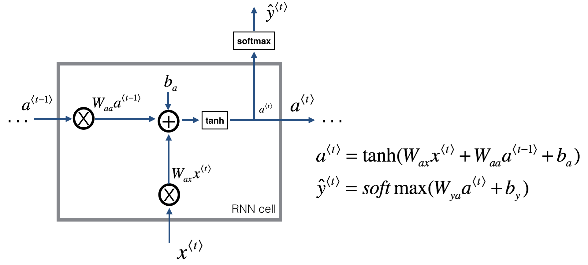
A Recurrent neural network can be seen as the repetition of a single cell (see $Figure\ 1$). Here we are first going to implement the computations for a single time-step. The following figure describes the operations for a single time-step of an RNN cell.

Figure 2: Basic RNN cell.

The above cell takes as input $x^{\langle t \rangle}$ (current input) and $a^{\langle t - 1\rangle}$ (previous hidden state containing information from the past), and outputs $a^{\langle t \rangle}$ which is given to the next RNN cell and also used to predict $y^{\langle t \rangle}$. Where tanh and softmax are two activation functions, which tanh is similar to sigmoid but more robust to usage scenarios, and softmax is a standard activation in classification problems.

You can see an RNN as the repetition of the cell you’ve just built. If your input sequence of data is carried over 10 time steps, then you will copy the RNN cell 10 times. Each cell takes as input the hidden state from the previous cell ($a^{\langle t-1 \rangle}$) and the current time-step’s input data ($x^{\langle t \rangle}$). It outputs a hidden state ($a^{\langle t \rangle}$) and a prediction ($y^{\langle t \rangle}$) for this time-step.

Figure 3: Basic RNN. The input sequence $x = (x^{\langle 1 \rangle}, x^{\langle 2 \rangle}, ..., x^{\langle T_x \rangle})$ is carried over $T_x$ time steps. The network outputs $y = (y^{\langle 1 \rangle}, y^{\langle 2 \rangle}, ..., y^{\langle T_x \rangle})$.

The KEY that this type of neural network can solve the problem of “How to avoid information inconsistence, i.e. the prediction may highly depends on the natural order (time series) of the data instead of given one input independently. “ For example, if we want to predict the next word of a sentence “他来自中国，他喜欢吃 ### “(“He comes from China, he loves(to eat) ###”).

As human, we read this sentence and extract information by sequence, first keyword: 吃(eat) tells us that this word should be noun. ranther than verb. or adv., and something related to eating, maybe a snack. And we look back to the second keyword 中国(China), which implies that this norn may related to Chinese food, so it is more reasonably to give an answer like 火锅(Hot Pot) than 电影(Movie) or 跑步(Running).

That’s exactly what we want machine to do. In RNN, given an input sequence, by adding extra information passed along entries by adding a term $a^{[t]}$ iterating neurons. While for the simple RNN, there is a problem called Gradient Vanishing or Explosion, which refers to tuning parameter matrix on $a^{[t]}$ in backpropagation could make the matrix exponentially decays to zero along sequence. i.e. Roughly speaking, makes the further information vanishes (can’t remember memory that’s too long ago). To solve this, we need something more subtle by controlling information update in the architecture LTSM or GRU.

LSTM

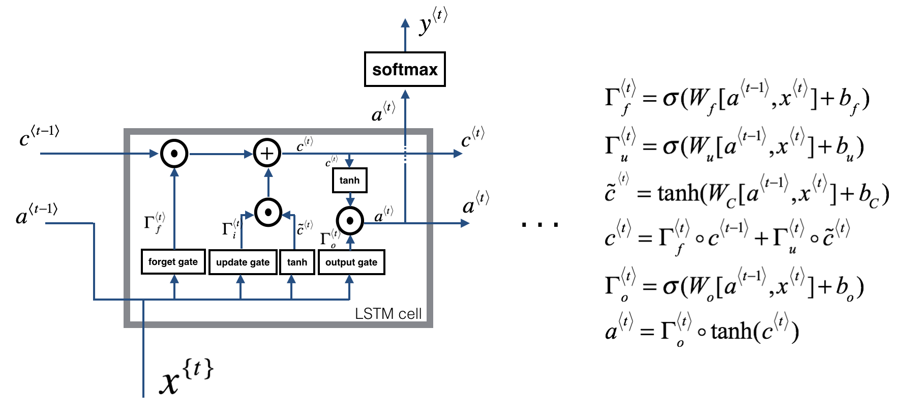
LSTM solves the problem mentioned above by adding gates to control the information update and what to pass into the next neuron. We post the Architecture of LSTM below:

Figure 4: LSTM-cell. This tracks and updates a "cell state" or memory variable $c^{\langle t \rangle}$ at every time-step, which can be different from $a^{\langle t \rangle}$.

About the Gates

• Forget Gate

  For the sake of this illustration, lets assume we are reading words in a piece of text, and want use an LSTM to keep track of grammatical structures, such as whether the subject is singular or plural. If the subject changes from a singular word to a plural word, we need to find a way to get rid of our previously stored memory value of the singular/plural state. In an LSTM, the forget gate lets us do this:

$$\Gamma_f^{\langle t \rangle} = \sigma(W_f[a^{\langle t-1 \rangle}, x^{\langle t \rangle}] + b_f)\tag{1}$$

Here, $W_f$ are weights that govern the forget gate's behavior. We concatenate $[a^{\langle t-1 \rangle}, x^{\langle t \rangle}]$ and multiply by $W_f$. The equation above results in a vector $\Gamma_f^{\langle t \rangle}$ with values between 0 and 1. This forget gate vector will be multiplied element-wise by the previous cell state $c^{\langle t-1 \rangle}$. So if one of the values of $\Gamma_f^{\langle t \rangle}$ is 0 (or close to 0) then it means that the LSTM should remove that piece of information (e.g. the singular subject) in the corresponding component of $c^{\langle t-1 \rangle}$. If one of the values is 1, then it will keep the information.

• Update Gate

  Once we forget that the subject being discussed is singular, we need to find a way to update it to reflect that the new subject is now plural. Here is the formulat for the update gate:

$$\Gamma_u^{\langle t \rangle} = \sigma(W_u[a^{\langle t-1 \rangle}, x^{\{t\}}] + b_u)\tag{2}$$

Similar to the forget gate, here $\Gamma_u^{\langle t \rangle}$ is again a vector of values between 0 and 1. This will be multiplied element-wise with $\tilde{c}^{\langle t \rangle}$, in order to compute $c^{\langle t \rangle}$.

• Updating the Cell
  To update the new subject we need to create a new vector of numbers that we can add to our previous cell state. The equation we use is: </p> $$\tilde{c}^{\langle t \rangle} = \tanh(W_c[a^{\langle t-1 \rangle}, x^{\langle t \rangle}] + b_c)\tag{3}$$

Finally, the new cell state is:

$$c^{\langle t \rangle} = \Gamma_f^{\langle t \rangle}* c^{\langle t-1 \rangle} + \Gamma_u^{\langle t \rangle} * \tilde{c}^{\langle t \rangle} \tag{4}$$

• Output Gate

  To decide which outputs we will use, we will use the following two formulas:

$$\Gamma_o^{\langle t \rangle}= \sigma(W_o[a^{\langle t-1 \rangle}, x^{\langle t \rangle}] + b_o)\tag{5}$$ $$a^{\langle t \rangle} = \Gamma_o^{\langle t \rangle}* \tanh(c^{\langle t \rangle})\tag{6}$$

Where in equation 5 you decide what to output using a sigmoid function and in equation 6 you multiply that by the $\tanh$ of the previous state.

Now that you have implemented one step of an LSTM, you can now iterate this over this using a for-loop to process a sequence of $T_x$ inputs.

Figure 5: LSTM over multiple time-steps.

Summary

Now we have come through RNN and LSTM, hopefully this post will prepare you the basic knowledge and intuition about how sequence model works. Using Keras library, we can simply build a deep learning models easily, numpy library also provides building-blocks for deep learning e.g. broadcasting to make Tensor Operation ( polynomial computation) hundreds of times faster than for-loop.

from keras import models
from keras import layers

# code snippet of constructing a simple network
# taking 10000 input points, with 3 hidden layers
# making binary classification

model = models.Sequential()
model.add(layers.Dense(64, activation='relu', input_shape=(10000,)))
model.add(layers.Dense(64, activation='relu'))
model.add(layers.Dense(2, activation='sigmoid'))
model.compile(optimizer='rmsprop',
              loss='catgorical_crossentropy',
              metrics=['accuracy'])

# train model!
model.fit(x_train,
          y_train,
          epocgs=10,
          batch_size=512,
          validation_data=(x_val, y_val))

In the following posts, I plan to add some basic Deep Learning knowledge (logistic regression, etc.), Environment Setup (Ubuntu, GPU, AWS cloud, etc.) and our final goal is to building a financial deep learning forecaster to construct trading strategies.

There are lots of resources that you can get access to online. I will recommend a book here: Deep Learning with Python, an amazing hands-on instructions for Keras library, you can’t even find a single math formula in Latex! since everything is written in programming language. (interpreted in loop) Despite the book, I would still suggest taking formal courses in order to better understand how deep learning works in algebra language. Also colah’s blog is a good place to learn, his posts were officially mentioned by Andrew Ng, especially this Understanding LSTM Networks, truly beautiful.

If you like this post, share it with your friends! XD